W14-W15. Differential Calculus
1. Theory
1.1 Introduction: Tangent Lines
When we look at the graph of a function, we often want to understand how it behaves at a specific point. One of the most important tools for this is the tangent line - a line that just “touches” the curve at a single point and has the same direction as the curve at that point.
1.1.1 The Slope of a Curve
Unlike a straight line which has a constant slope, a curved function has a slope that changes from point to point. To find the slope of a curve at a specific point
- Take a nearby point
- Draw the secant line connecting
- Calculate the slope of this secant line:
- Let point
- The limiting value of these slopes is the slope of the tangent line
This gives us the formula:
The expression
Example: For the function
This slope is always negative for
1.1.2 Vertical Tangent Lines
Sometimes a curve can have a vertical tangent line at a point. This occurs when the limit of the difference quotient exists but equals
Example: The function
However, not all functions with vertical-looking behavior at a point have vertical tangent lines. The function
1.2 The Derivative at a Point
The concept of the slope of a tangent line leads us to one of the most fundamental ideas in calculus: the derivative.
1.2.1 Definition of the Derivative at a Point
Let
provided this limit exists and is finite.
Alternative notations for the derivative at
We can also write this definition using a different variable substitution. If we set
The derivative
1.3 The Derivative as a Function
Instead of finding the derivative at just one specific point, we can find the derivative at every point where it exists, creating a new function called the derivative function.
1.3.1 Definition of the Derivative Function
The derivative of
provided the limit exists.
The domain of
If
Examples of computing derivatives from the definition:
- For
- For
- For
1.3.2 One-Sided Derivatives and Differentiability on Intervals
A function can have different behaviors when approached from the left versus the right at a point. This leads to the concept of one-sided derivatives.
For a function
- The right-hand derivative at
- The left-hand derivative at
A function
- Differentiable on an open interval if it has a derivative at each point of the interval
- Differentiable on a closed interval
Important: A function has a derivative at an interior point if and only if both the left-hand and right-hand derivatives exist there and are equal.
Example: The function
- Right-hand derivative:
- Left-hand derivative:
Since these are different,
1.4 Differentiability and Continuity
There’s an important relationship between differentiability and continuity: differentiable functions are always continuous, but continuous functions are not always differentiable.
1.4.1 Theorem: Differentiability Implies Continuity
Theorem: If
Proof: We need to show that
Taking limits as
This proves continuity at
Important: The converse is not true. The function
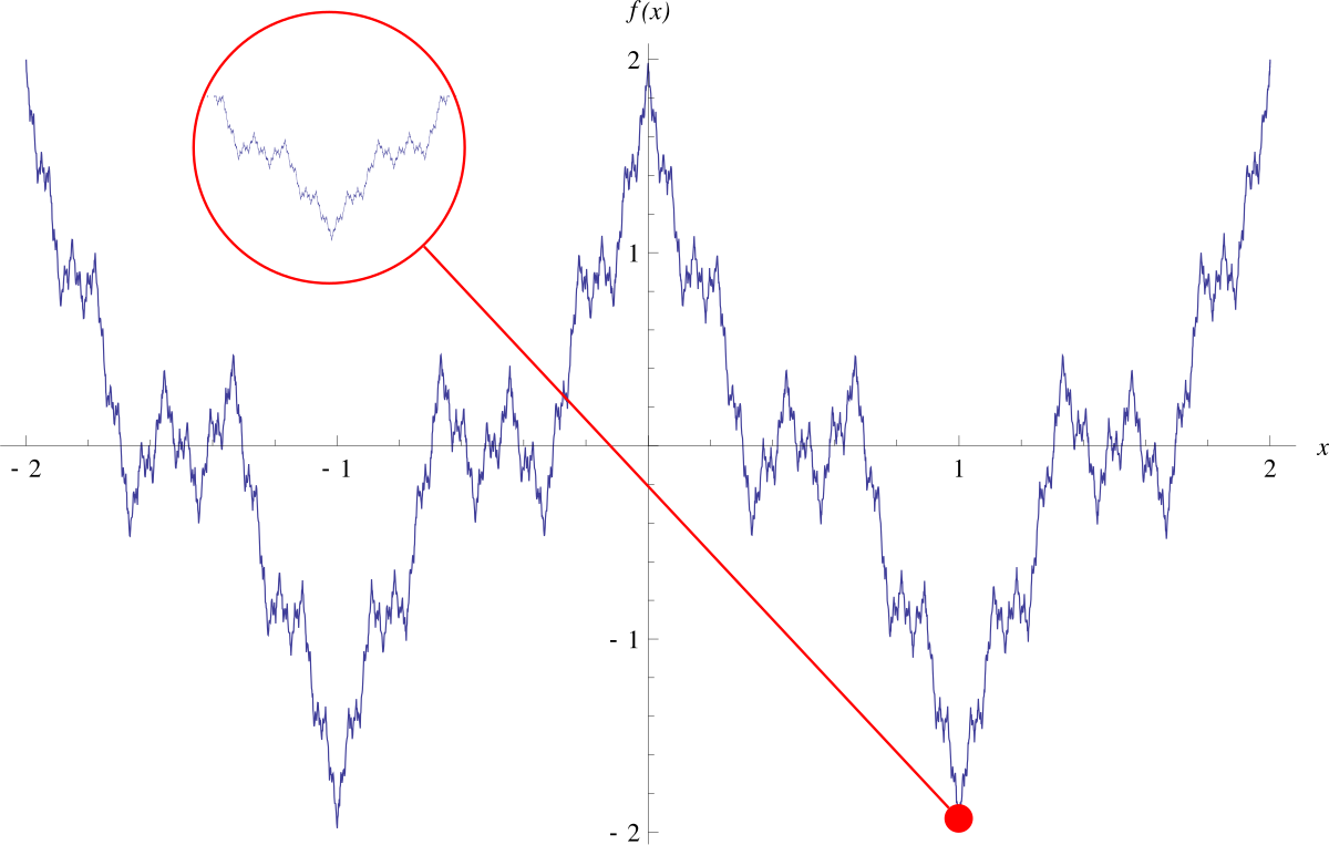
1.4.2 Nowhere Differentiable Functions
It’s possible for a function to be continuous everywhere but differentiable nowhere! A famous example is the Weierstrass function:
where
1.5 Differentiation Rules
Computing derivatives using the definition (the limit process) can be tedious. Fortunately, we have differentiation rules that allow us to find derivatives quickly and efficiently.
1.5.1 Basic Rules
Constant Multiple Rule: If
Proof: By definition,
Sum Rule: If
Proof: By definition:
Difference Rule: Combining the Sum Rule with the Constant Multiple Rule gives:
These rules extend to sums of more than two functions by mathematical induction.
1.5.2 Product and Quotient Rules
Product Rule: If
Proof: Starting from the definition:
We add and subtract
Since
Quotient Rule: If
Proof: By definition:
Adding and subtracting
1.6 Derivatives of Elementary Functions
Using the definition of the derivative and the rules above, we can derive formulas for all elementary functions.
1.6.1 Constant and Power Functions
Derivative of a Constant: If
Power Rule: For any real number
Proof for positive integers: We use the algebraic identity:
From the definition:
(There are
The proof for general real
1.6.2 Exponential Functions
Derivative of Exponential Functions: For
Proof: We use the important limit
Special case: For the natural exponential function:
This is one of the most remarkable properties of
1.6.3 Trigonometric Functions
Derivative of Sine: Using the angle addition formula and important limits
Derivative of Cosine: Similarly:
Other Trigonometric Functions: Using the Quotient Rule:
1.7 The Chain Rule
When we have a composite function (a function inside another function), we need a special rule to find its derivative.
1.7.1 The Chain Rule Theorem
Theorem (The Chain Rule): If
In other words: the derivative of the outer function (evaluated at the inner function) times the derivative of the inner function.
Alternative notation: If we set
The Chain Rule tells us that the rate of change at
1.7.2 Chain Rule for Elementary Functions
Applying the Chain Rule to our elementary functions (where
Examples:
1.8 Derivatives of Inverse Functions
When a function has an inverse, there’s a beautiful relationship between their derivatives.
1.8.1 The Inverse Function Rule
Theorem: Let
Moreover, if
Proof sketch: From
Therefore:
Example: Let
1.8.2 Derivative of the Natural Logarithm
Since
Therefore:
By the Chain Rule, for a positive differentiable function
Examples:
1.8.3 Derivatives of Inverse Trigonometric Functions
Derivative of
Therefore:
With Chain Rule:
Derivative of
Derivative of
Therefore:
Other inverse trigonometric functions:
1.9 Logarithmic Differentiation
For functions involving products, quotients, and powers, taking the logarithm before differentiating can greatly simplify the calculation. This technique is called logarithmic differentiation.
Example: To find the derivative of
- Take the natural logarithm of both sides:
- Differentiate both sides (using
- Solve for
1.9.1 Derivatives of the Form
For functions where both the base and exponent depend on
Examples:
- For
- For
- For
1.10 Higher-Order Derivatives
If the derivative
1.10.1 Notation for Higher-Order Derivatives
The
For the first few derivatives:
- First derivative:
- Second derivative:
- Third derivative:
- Fourth derivative:
1.10.2 Leibniz Formula for the
There’s a formula analogous to the binomial theorem for the
where
1.10.3 Examples of Higher-Order Derivatives
Example 1: For
We can see a pattern and prove by induction that:
Example 2: For
The pattern repeats with period 4. By induction, we can prove:
Similarly,
Other useful formulas:
1.11 Indeterminate Forms and L’Hôpital’s Rule
When evaluating limits, we often encounter expressions that don’t have an obvious value. These are called indeterminate forms.
1.11.1 Indeterminate Forms
The common indeterminate forms are:
Each requires special techniques to evaluate. The most powerful technique is L’Hôpital’s Rule.
1.11.2 L’Hôpital’s Rule
Theorem (L’Hôpital’s Rule): Suppose
or
Then:
provided the limit on the right side exists (or is
Important notes:
- L’Hôpital’s Rule says: differentiate the numerator and denominator separately, then take the limit
- The rule applies to one-sided limits and limits at infinity (replace
- Only use when you have an indeterminate form! For example,
Why it works (special case): When
1.11.3 Examples Using L’Hôpital’s Rule
Type
Type
Type
Type
1.11.4 Indeterminate Powers:
For limits of the form
- Take the logarithm:
- Rewrite as an exponential:
Both lead to evaluating the indeterminate product
Example 1:
Let
Therefore:
Example 2:
We write
1.11.5 When L’Hôpital’s Rule Doesn’t Help
Sometimes L’Hôpital’s Rule leads to an infinite loop or more complicated expressions. In such cases, use algebraic manipulation instead.
Example 1:
L’Hôpital’s Rule keeps cycling. Instead, divide numerator and denominator by
Example 2:
L’Hôpital’s Rule keeps producing similar forms. Instead, divide by the dominant term
As
As
1.12 Taylor Series and Taylor’s Theorem
One of the most powerful ideas in calculus is representing functions as infinite series. This allows us to approximate complicated functions with polynomials and use them to calculate limits and analyze function behavior.
1.12.1 Motivation: Approximating Functions with Polynomials
Polynomials are the simplest functions to work with - they only involve addition and multiplication. Can we approximate more complicated functions (like
Consider approximating
For example,
Where does this approximation come from? It’s the second-degree Taylor polynomial of
1.12.2 Power Series Representations
A power series centered at
Theorem (Term-by-Term Differentiation): If a power series
on the interval
Important consequence: Within its interval of convergence, a power series sum is infinitely differentiable.
Question: If
1.12.3 Determining the Coefficients
Suppose
with positive radius of convergence. Differentiating term by term:
In general, for the
Evaluating at
Therefore:
Conclusion: If
1.12.4 Taylor Series and Maclaurin Series
Definition: Let
When
The Taylor polynomial of order
Example: For
- General pattern:
The Maclaurin series is:
The Taylor polynomials are:
1.12.5 Taylor’s Theorem and the Remainder
Important question: When does the Taylor series actually equal the function? Not always!
Taylor’s Theorem: If
where
for some
Convergence condition:
In that case:
Example: For
Since
for some
- If
- If
In both cases,
Therefore:
Setting
1.12.6 Frequently Used Taylor/Maclaurin Series
Here are the most important series (all at
Exponential and Logarithmic:
Trigonometric:
Hyperbolic:
Inverse Trigonometric:
Powers and Fractions:
where
1.12.7 Using Taylor Series to Find Limits
Taylor series are extremely useful for calculating limits, especially when L’Hôpital’s Rule becomes complicated.
Asymptotic notation:
Example 1: Calculate
Using Taylor series:
Therefore:
So:
Example 2: Calculate
First:
For the base:
Therefore:
using the limit
1.13 Applications: Extreme Values of Functions
One of the most important applications of derivatives is finding the maximum and minimum values of functions - crucial in optimization problems across science, engineering, and economics.
1.13.1 Types of Extreme Values
Definitions: Let
- An absolute (global) maximum of
- An absolute (global) minimum of
- A local (relative) maximum of
- A local (relative) minimum of
Absolute extrema are “global” - they’re the highest/lowest values over the entire domain. Local extrema are “neighborhood” - they’re highest/lowest in some small region around the point.
1.13.2 The Extreme Value Theorem
Theorem (Extreme Value Theorem): If
This theorem is intuitively clear but requires deep knowledge of real numbers to prove rigorously.
Important: All three conditions are essential:
- Closed interval: On
- Bounded interval: On
- Continuity: On
1.13.3 Fermat’s Theorem
Theorem (Fermat’s Theorem): If
Proof: Suppose
From the right:
From the left:
Since both limits must equal
Important notes:
- The converse is false:
- Extrema can occur where
1.13.4 Critical Points
Definition: An interior point of the domain of
Key result: If
- A critical point, or
- An endpoint of the domain
This gives us a strategy for finding extreme values:
- Find all critical points (where
- Evaluate
- The largest value is the absolute maximum, the smallest is the absolute minimum
Example: For
Critical points:
Evaluate:
Absolute max:
1.14 The Mean Value Theorem
The Mean Value Theorem is one of the most important theoretical tools in calculus, with far-reaching consequences.
1.14.1 Rolle’s Theorem
Theorem (Rolle’s Theorem): Suppose
Geometric interpretation: If a differentiable curve starts and ends at the same height, there must be at least one point where the tangent is horizontal.
Proof: By the Extreme Value Theorem,
- If both occur at endpoints, then
- If either occurs at an interior point
1.14.2 The Mean Value Theorem
Theorem (Mean Value Theorem): Suppose
Geometric interpretation: There exists a point where the tangent line is parallel to the secant line connecting the endpoints.
Proof: Consider the function:
This measures the vertical distance between
1.14.3 Consequences of the Mean Value Theorem
Corollary 1: If
Proof: For any
Corollary 2: If
Proof: Apply Corollary 1 to
Corollary 3 (Monotonicity Test):
- If
- If
Proof: For
for some
- If
- If
1.15 The First and Second Derivative Tests
The derivative tests give us practical methods for classifying critical points.
1.15.1 First Derivative Test
Theorem (First Derivative Test): Suppose
- If
- If
- If
Example: For
Critical points:
| Interval | |||
|---|---|---|---|
| Sign of |
|||
| Behavior | decreasing | decreasing | increasing |
Therefore: no extremum at
1.15.2 Concavity
Definition: The graph of a differentiable function
- Concave up (convex) on interval
- Concave down on interval
Second Derivative Test for Concavity:
- If
- If
Definition: A point
1.15.3 Second Derivative Test
Theorem (Second Derivative Test): Suppose
- If
- If
- If
Proof of (1): Since
Why the test can fail when
1.16 Curve Sketching
Combining our tools, we can sketch accurate graphs of functions.
1.16.1 Curve Sketching Procedure
- Domain and symmetry: Find the domain and check for symmetry (even/odd functions)
- Asymptotes: Find vertical, horizontal, and oblique asymptotes
- Derivatives: Calculate
- Critical points: Find where
- Monotonicity: Determine where
- Concavity and inflection points: Determine where
- Plot key points: Mark intercepts, critical points, inflection points, and sketch
1.16.2 Example
Sketch
Domain:
Asymptotes:
Derivatives:
Critical points:
Monotonicity:
Interval Sign of Behavior decreasing increasing decreasing Local minimum at
Concavity:
Sketch: Plot the key points and connect smoothly, respecting the monotonicity and concavity.
2. Definitions
- Tangent Line: A line that touches a curve at a single point and has the same slope as the curve at that point. For the curve
- Difference Quotient: The expression
- Vertical Tangent Line: A curve has a vertical tangent line at
- Derivative at a Point: The derivative of
- Derivative Function: The function
- Differentiable at a Point: A function
- Differentiable on an Interval: A function is differentiable on an open interval if it has a derivative at each point; differentiable on a closed interval
- Right-Hand Derivative: The limit
- Left-Hand Derivative: The limit
- Critical Point: An interior point
- Increasing Function: A function
- Decreasing Function: A function
- Concave Up (Convex): A differentiable function
- Concave Down: A differentiable function
- Inflection Point: A point
- Absolute (Global) Maximum: A value
- Absolute (Global) Minimum: A value
- Local (Relative) Maximum: A value
- Local (Relative) Minimum: A value
- Higher-Order Derivatives: The
- Indeterminate Form: An expression arising in limit evaluation that doesn’t have an obvious value, such as
- Taylor Series: The series
- Maclaurin Series: A Taylor series centered at
- Taylor Polynomial: The polynomial
- Remainder (Taylor’s Theorem): The term
- Logarithmic Differentiation: A technique where we take the natural logarithm of both sides of an equation before differentiating, useful for products, quotients, and variable exponents.
- Convex Function (without differentiability): A function
- Strictly Convex Function: A convex function where the inequality is strict whenever
3. Formulas
Basic Differentiation Rules:
- Constant Rule:
- Power Rule:
- Constant Multiple Rule:
- Sum Rule:
- Difference Rule:
- Product Rule:
- Quotient Rule:
- Chain Rule:
Derivatives of Elementary Functions:
- Exponential Functions:
- Logarithmic Functions:
- Trigonometric Functions:
- Inverse Trigonometric Functions:
- Hyperbolic Functions:
Chain Rule Forms (where
Inverse Function Rule:
Higher-Order Derivatives:
- Leibniz Formula:
- Common Higher Derivatives:
L’Hôpital’s Rule:
- If
Taylor Series (Maclaurin Series at
- General Formula:
- Taylor’s Formula:
- Common Series:
Theorems and Tests:
- Fermat’s Theorem: If
- Rolle’s Theorem: If
- Mean Value Theorem: If
- Monotonicity Test:
- First Derivative Test: At critical point
- Second Derivative Test: If
- Concavity Test:
4. Practice
4.1. Limit with Indeterminate Form
Calculate the limit:
Click to see the solution
Key Concept: This is an indeterminate form
- Rewrite using exponential form:
- Find the limit of the exponent:
- Use Taylor series or L’Hôpital’s Rule: As
- Compute the limit:
Answer:
4.2. Limit with Indeterminate Form
Calculate the limit:
Click to see the solution
Key Concept: This is an indeterminate form
- Rewrite using exponential form:
- Simplify the base:
- Find the limit of the exponent:
- Evaluate each term:
- Compute the limit:
Answer:
4.3. Taylor Polynomials for
Find the Taylor Polynomials of orders 1, 2, and 3 generated by
Click to see the solution
Key Concept: Use the formula
- Find derivatives:
- Construct Taylor polynomials:
- Order 1:
- Order 2:
- Order 3:
- Order 1:
Answer:
4.4. Taylor Polynomials for
Find the Taylor Polynomials of orders 1, 2, and 3 generated by
Click to see the solution
Key Concept: Use the formula
- Find derivatives:
- Construct Taylor polynomials:
- Order 1:
- Order 2:
- Order 3:
- Order 1:
Answer:
4.5. Taylor Series for
Find the Taylor series generated by
Click to see the solution
Key Concept: Use the formula
- Find derivatives: Since
- Construct the Taylor series:
- Simplify:
Answer:
4.6. Taylor Series for
Find the Taylor series generated by
Click to see the solution
Key Concept: Use the formula for geometric series or find derivatives directly.
- Method 1: Using geometric series: Write
- Method 2: Using derivatives:
Answer:
4.7. Limit Using Taylor Series (Lab 15, Task 7)
Calculate the limit:
Click to see the solution
Key Concept: Expand each term using Taylor series (Maclaurin series) at
Expand each function:
Compute the numerator:
- Therefore:
Compute the denominator:
Compute the limit:
Answer:
4.8. Analyze Variation and Sketch the Graph (Lab 15, Task 8)
Study the variation and graph of the function:
Click to see the solution
Key Concept: Analyze domain, symmetry, asymptotes, derivatives, and monotonicity to sketch the graph.
- Domain: We need
- Symmetry:
- Asymptotes:
- As
- By symmetry,
- No vertical asymptotes (function is continuous on its domain).
- As
- First derivative:
- Critical points:
- Behavior at endpoints:
- As
- As
- Second derivative (for concavity):
Answer: The function is even, defined on
4.9. Find the Slope of a Curve at Any Point (Chapter 6, Example 1)
Find the slope of the curve
Click to see the solution
Key Concept: Use the definition of the derivative to find the slope at any point.
- Apply the definition: We have
- Simplify the numerator:
- Cancel and evaluate:
- Find where slope equals
Answer: The slope at
Note: The slope is always negative for
4.10. Compute Derivatives from the Definition (Chapter 6, Example 2)
By the definition, find the derivative of the following functions:
(a)
(b)
(c)
(d)
Click to see the solution
(a)
- Apply the definition:
- Simplify:
- Evaluate:
Answer (a):
(b)
- Apply the definition:
- Expand:
- Simplify:
Answer (b):
(c)
- Apply the definition:
- Rationalize:
- Evaluate:
Answer (c):
(d)
- Apply the definition:
- Combine fractions:
- Expand and simplify:
- Evaluate:
Answer (d):
4.11. Evaluate a Limit Using Taylor Series (Chapter 6, Example 3)
Calculate
Click to see the solution
Key Concept: This is type
- Expand the exponent:
- Expand the base:
- Compute the limit:
Answer:
4.12. Apply Differentiation Rules (Chapter 6, Example 4)
Find the derivatives of the following functions:
(a)
(b)
(c)
(d)
Click to see the solution
(a)
Answer (a):
(b)
- Derivative of first term:
- Derivative of second term (quotient rule):
Answer (b):
(c)
- First term (product rule):
- Second term (power rule):
- Third term:
Answer (c):
Note:
(d)
- First term (product rule):
- Second term (product rule):
Answer (d):
4.13. Differentiate Composite and Rational Functions (Chapter 6, Example 5)
Find the derivatives of the following functions:
(a)
(b)
(c)
(d)
(e)
(f)
Click to see the solution
(a)
Using the quotient rule, or first expand numerator and denominator:
Numerator:
Denominator:
After simplification:
Answer (a):
(b)
Using quotient rule:
Answer (b):
(c)
Using product rule:
Answer (c):
(d)
Using quotient rule:
Answer (d):
(e)
Answer (e):
(f)
Using quotient rule (or chain rule with product):
Answer (f):
4.14. Chain Rule Applications (Chapter 6, Example 6)
Find the derivatives:
(a)
(b)
(c)
Click to see the solution
(a): Using chain rule:
Answer (a):
(b): Using product rule multiple times:
Answer (b):
(c): Using chain rule:
Answer (c):
4.15. Derivative of Inverse Function (Chapter 6, Example 7)
Let
Click to see the solution
Key Concept: Use the inverse function rule:
- Identify the values: We have
- Find
- Evaluate
- Apply the inverse function rule:
Answer:
4.16. Logarithmic Differentiation (Chapter 6, Example 8)
Find the derivative of
Click to see the solution
Key Concept: Take the logarithm of both sides before differentiating to simplify products and quotients.
- Take the natural logarithm:
- Differentiate both sides:
- Solve for
Answer:
4.17. Derivatives of
Find the derivatives:
(a)
(b)
(c)
Click to see the solution
Key Concept: For
(a)
- Rewrite:
- Differentiate:
Answer (a):
(b)
- Rewrite:
- Differentiate:
Answer (b):
(c)
- Rewrite:
- Differentiate the exponent:
- Apply chain rule:
Answer (c):
4.18. Find the
Find the
Click to see the solution
- Compute the first few derivatives:
- Identify the pattern:
- Prove by induction: Base case (
Answer:
4.19. L’Hôpital’s Rule Examples (Chapter 6, Example 11)
Calculate the following limits using L’Hôpital’s Rule:
(a)
(b)
(c)
(d)
(e)
Click to see the solution
(a) Type
Answer (a):
(b) Type
This is still
Answer (b):
(c) Type
Answer (c):
(d) Type
Answer (d):
(e) Type
Type
Still
Answer (e):
4.20. Indeterminate Powers (Chapter 6, Example 12)
Calculate:
(a)
(b)
Click to see the solution
(a) Type
Let
Therefore:
Answer (a):
(b) Type
Write
Answer (b):
4.21. Sum of Series Using
Given that
(a)
(b)
Click to see the solution
(a) Split the sum:
For the first sum, note that
For the second sum:
Therefore:
Answer (a):
(b) Split the sum:
For
Therefore:
Answer (b):
4.22. Find Limits Using Taylor Series (Chapter 6, Example 14)
Calculate
Click to see the solution
Key Concept: Use Taylor series expansions around
- Expand each function:
- Compute numerator:
- Compute the limit:
Answer:
4.23. Find Absolute Extrema on a Closed Interval (Chapter 6, Example 15)
(a) Find the absolute maximum and minimum values of
(b) Find the absolute maximum and minimum values of
Click to see the solution
(a)
- Find critical points:
- Evaluate
- Identify extrema:
- Absolute maximum:
- Absolute minimum:
- Absolute maximum:
Answer (a): Absolute max:
(b)
- Find critical points:
- Evaluate
- Identify extrema:
- Absolute maximum:
- Absolute minimum:
- Absolute maximum:
Answer (b): Absolute max:
4.24. First Derivative Test (Chapter 6, Example 16)
(a) For
(b) For
Click to see the solution
(a)
Find
Find critical points:
Test sign of
Interval Sign of Behavior decreasing decreasing increasing Classify critical points:
- At
- At
- At
Answer (a): Critical points:
(b)
Find
Find critical points:
Test sign of
Interval Sign of Behavior increasing decreasing increasing Classify critical points:
- At
- At
- At
Answer (b): Local max at
4.25. Curve Sketching: Example 1 (Chapter 6, Example 17)
Sketch the graph of
Click to see the solution
Domain:
Asymptotes:
First derivative:
Monotonicity:
Interval Sign of Behavior decreasing increasing decreasing - Local minimum at
- Local maximum at
- Local minimum at
Second derivative:
Concavity:
Interval Sign of Concavity up down up down Key points:
- Intercepts:
- Inflection points at
- Intercepts:
Answer: See sketch with horizontal asymptote
4.26. Curve Sketching: Example 2 (Chapter 6, Example 18)
Sketch the graph of
Click to see the solution
Domain:
Limits and asymptotes:
First derivative:
Second derivative:
Concavity:
Interval Sign of Concavity down up up
Answer: See sketch with vertical asymptote at
4.27. Curve Sketching: Example 3 (Chapter 6, Example 19)
Sketch the graph of
Click to see the solution
Domain:
Limits:
First derivative:
Monotonicity:
Interval Sign of Behavior increasing increasing decreasing decreasing - At
- At
- At
- At
Second derivative:
Concavity:
Interval Sign of Concavity up down down
Answer: See sketch with cusp at origin
4.28. Find the Sum of Series
Find the sum:
Click to see the solution
Key Concept: Use partial fractions and telescoping series.
- Factor the denominator:
- Use partial fractions:
- Write partial sum:
- Take limit:
Answer:
4.29. Limits Without L’Hôpital - Problem 1 (Preparing for Final, Limits 1)
Evaluate (without using L’Hôpital’s Rule):
Click to see the solution
Key Concept: Factor numerator and denominator.
- Factor:
- Simplify:
- Evaluate:
Answer:
4.30. Limits Without L’Hôpital - Problem 2 (Preparing for Final, Limits 1)
Evaluate (without using L’Hôpital’s Rule):
Click to see the solution
Key Concept: Factor numerator. Since
- Factor numerator: Using polynomial division or synthetic division:
- Simplify:
Answer:
4.31. Limits Without L’Hôpital - Problem 3 (Preparing for Final, Limits 1)
Evaluate (without using L’Hôpital’s Rule):
Click to see the solution
Key Concept: Rationalize the numerator.
- Rationalize:
- Evaluate:
Answer:
4.32. Limits Without L’Hôpital - Problem 4 (Preparing for Final, Limits 1)
Evaluate (without using L’Hôpital’s Rule):
Click to see the solution
Key Concept: Use the identity
- Rationalize using cube root identity: Let
- Evaluate:
Answer:
4.33. Derivative by Definition - Problem 1 (Preparing for Final, Differentiation 1)
By the definition, find the derivative of:
Click to see the solution
Key Concept: Use the definition
- Apply the definition:
- Combine fractions:
- Expand and simplify: Numerator:
- Evaluate:
Answer:
4.34. Derivative by Definition - Problem 2 (Preparing for Final, Differentiation 1)
By the definition, find the derivative of:
Click to see the solution
Key Concept: Use the definition of the derivative.
- Apply the definition:
- Expand:
Answer:
4.35. Find the Sum of Series
Find the sum:
Click to see the solution
Key Concept: Use partial fractions and telescoping series.
- Use partial fractions:
- Write partial sum and take limit: The series telescopes, and after taking the limit:
Answer:
4.36. Limits Without L’Hôpital - Problem 5 (Preparing for Final, Limits 2)
Find the limit (without using L’Hôpital’s Rule):
Click to see the solution
Key Concept: Consider left and right limits separately due to absolute value.
- Right limit (
- Left limit (
- Conclusion: Since the left and right limits differ, the limit does not exist.
Answer: Limit does not exist
4.37. Limits Without L’Hôpital - Problem 6 (Preparing for Final, Limits 2)
Find the limit (without using L’Hôpital’s Rule):
Click to see the solution
Key Concept: Rationalize the numerator.
- Rationalize:
- Evaluate:
Answer:
4.38. Limits Without L’Hôpital - Problem 7 (Preparing for Final, Limits 2)
Find the limit (without using L’Hôpital’s Rule):
Click to see the solution
Key Concept: Use the limit
- Rewrite:
- Evaluate:
Answer:
4.39. Limits Without L’Hôpital - Problem 8 (Preparing for Final, Limits 2)
Find the limit (without using L’Hôpital’s Rule):
Click to see the solution
Key Concept: Use substitution and known limits.
- Substitute
- Rewrite:
Answer:
4.40. Limits Without L’Hôpital - Problem 9 (Preparing for Final, Limits 2)
Find the limit (without using L’Hôpital’s Rule):
Click to see the solution
Key Concept: Use substitution and known limits.
- Substitute
- Rewrite:
Answer:
4.41. Limits Without L’Hôpital - Problem 10 (Preparing for Final, Limits 2)
Find the limit (without using L’Hôpital’s Rule):
Click to see the solution
Key Concept: Rewrite in terms of sine and cosine, then use known limits.
- Rewrite:
- Use known limits:
Answer:
4.42. Limits Without L’Hôpital - Problem 11 (Preparing for Final, Limits 2)
Find the limit (without using L’Hôpital’s Rule):
Click to see the solution
Key Concept: Factor and use known limits.
- Factor:
- Use known limits:
Answer:
4.43. Limits Without L’Hôpital - Problem 12 (Preparing for Final, Limits 2)
Find the limit (without using L’Hôpital’s Rule):
Click to see the solution
Key Concept: Rewrite in terms of sine and cosine, then use known limits.
- Rewrite:
- Use known limits:
Answer:
4.44. Logarithmic Differentiation (Preparing for Final, Differentiation 2)
Find the derivative of the function
Click to see the solution
Key Concept: Use logarithmic differentiation.
- Take natural logarithm:
- Differentiate both sides:
- Solve for
Answer:
4.45. Find the Sum of Series
Find the sum:
Click to see the solution
Key Concept: This is a telescoping series.
- Use partial fractions:
- Write partial sum:
- Take limit:
Answer:
4.46. Limits at Infinity - Problem 1 (Preparing for Final, Limits 3)
Find (without using L’Hôpital’s Rule):
Click to see the solution
Key Concept: Divide by the dominant exponential term.
- Divide numerator and denominator by
- Evaluate: As
Answer:
4.47. Limits at Infinity - Problem 2 (Preparing for Final, Limits 3)
Find (without using L’Hôpital’s Rule):
Click to see the solution
Key Concept: Divide by the dominant exponential term. As
- Divide numerator and denominator by
- Evaluate: As
Answer:
4.48. Limits at Infinity - Problem 3 (Preparing for Final, Limits 3)
Find (without using L’Hôpital’s Rule):
Click to see the solution
Key Concept: Substitute
- Substitute
- Rewrite:
- Evaluate: Since
Answer:
4.49. Limits at Infinity - Problem 4 (Preparing for Final, Limits 3)
Find (without using L’Hôpital’s Rule):
Click to see the solution
Key Concept: Divide by the highest power of
Divide numerator and denominator by
Simplify exponents:
Evaluate: As
- All other terms approach
Answer:
4.50. Limits at Infinity - Problem 5 (Preparing for Final, Limits 3)
Find (without using L’Hôpital’s Rule):
Click to see the solution
Key Concept: Rationalize the expression.
- Rationalize:
- Evaluate: As
Answer:
4.51. Limits at Infinity - Problem 6 (Preparing for Final, Limits 3)
Find (without using L’Hôpital’s Rule):
Click to see the solution
Key Concept: Rationalize the expression.
- Rationalize:
- Evaluate: As
Answer:
4.52. Taylor Polynomials for
Find the Taylor Polynomials of orders 1, 2, and 3 generated by
Click to see the solution
Key Concept: Compute derivatives and use Taylor polynomial formula.
- Find derivatives:
- Construct Taylor polynomials:
Answer:
4.53. Taylor Polynomials for
Find the Taylor Polynomials of orders 1, 2, and 3 generated by
Click to see the solution
Key Concept: Compute derivatives at
- Find derivatives at
- Construct Taylor polynomials:
Answer:
4.54. Taylor Polynomials for
Find the Taylor Polynomials of orders 1, 2, and 3 generated by
Click to see the solution
Key Concept: Compute derivatives at
- Find derivatives:
- Construct Taylor polynomials:
Answer:
4.55. Find the Sum of Series
Find the sum:
Click to see the solution
Key Concept: This is a telescoping series.
- Write partial sum:
- Take limit: Since
Answer:
4.56. Limits with Indeterminate Powers - Problem 1 (Preparing for Final, Limits 4)
Find the limit:
Click to see the solution
Key Concept: This is type
- Rewrite:
- Find limit of exponent:
- Compute the limit:
Answer:
4.57. Limits with Indeterminate Powers - Problem 2 (Preparing for Final, Limits 4)
Find the limit:
Click to see the solution
Key Concept: Type
- Rewrite:
- Find limit of exponent:
Answer:
4.58. Limits with Indeterminate Powers - Problem 3 (Preparing for Final, Limits 4)
Find the limit:
Click to see the solution
Key Concept: Type
- Rewrite:
- Find limit of exponent:
- Compute the limit:
Answer:
4.59. Limits with Indeterminate Powers - Problem 4 (Preparing for Final, Limits 4)
Find the limit:
Click to see the solution
Key Concept: Type
- Substitute
- Rewrite:
- Use exponential form:
- Find limit of exponent: As
- Compute the limit:
Answer:
4.60. Taylor Series for
Find the Taylor series of
Click to see the solution
Key Concept: Use geometric series or find derivatives.
- Method 1: Geometric series:
- Method 2: Derivatives:
Answer:
4.61. Taylor Series for
Find the Taylor series of
Click to see the solution
Key Concept: Use geometric series with substitution.
- Rewrite:
- Use geometric series: For
Answer:
4.62. Taylor Series for
Find the Taylor series of
Click to see the solution
Key Concept: Use geometric series with substitution.
- Rewrite:
- Use geometric series: For
Answer:
4.63. Taylor Series for
Find the Taylor series of
Click to see the solution
Key Concept: Use known series for
- Use known series:
- Multiply by
Answer:
4.64. Taylor Series for
Find the Taylor series of
Click to see the solution
Key Concept: Use substitution and known series.
- Substitute
- Use series for
- Multiply:
Answer:
4.65. Taylor Series for
Find the Taylor series of
Click to see the solution
Key Concept: Use known series for
- Use known series:
- Multiply by
Answer:
4.66. Taylor Series for
Find the Taylor series of
Click to see the solution
Key Concept: Use substitution and known series.
- Substitute
- Use series for
- Multiply and combine:
Answer:
4.67. Find the Sum of Series
Find the sum:
Click to see the solution
Key Concept: This is a telescoping series.
- Write partial sum:
- Take limit:
Answer:
4.68. Limit Using Taylor Series - Problem 1 (Preparing for Final, Differentiation 5)
Find the limit:
Click to see the solution
Key Concept: Use Taylor series expansions. (This problem was solved in Example 4.13, answer is
- Expand each function:
- Compute numerator:
- Compute the limit:
Answer:
4.69. Limit Using Taylor Series - Problem 2 (Preparing for Final, Differentiation 5)
Find the limit:
Click to see the solution
Key Concept: Use Taylor series expansions. (This problem was solved in Lab 15 Problem 7, but answer given is
- Expand each function:
- Compute numerator:
- Compute denominator:
- Compute the limit:
Answer:
4.70. Find the Sum of Series
Find the sum:
Click to see the solution
Key Concept: This is a geometric series.
- Rewrite:
- Use geometric series formula: For
Answer:
4.71. Sketch Graph - Problem 1 (Preparing for Final, Differentiation 6)
Sketch the graph of:
Click to see the solution
Key Concept: This problem was solved in detail in Example 4.17. See that solution for complete analysis.
Answer: See Example 4.17 for complete solution. Key features: horizontal asymptote
4.72. Sketch Graph - Problem 2 (Preparing for Final, Differentiation 6)
Sketch the graph of:
Click to see the solution
Key Concept: This problem was solved in detail in Example 4.18. See that solution for complete analysis.
Answer: See Example 4.18 for complete solution. Key features: vertical asymptote at
4.73. Sketch Graph - Problem 3 (Preparing for Final, Differentiation 6)
Sketch the graph of:
Click to see the solution
Key Concept: This problem was solved in detail in Example 4.19. See that solution for complete analysis.
Answer: See Example 4.19 for complete solution. Key features: cusp at origin
4.74. Sketch Graph - Problem 4 (Preparing for Final, Differentiation 6)
Sketch the graph of:
Click to see the solution
Key Concept: Analyze domain, asymptotes, derivatives, and behavior.
- Domain:
- Asymptotes:
- Vertical:
- Oblique: Perform division:
- No horizontal asymptote
- Vertical:
- Derivatives and critical points:
- Behavior:
- Local max at
Answer: See sketch with vertical asymptotes at
4.75. Sketch Graph - Problem 5 (Preparing for Final, Differentiation 6)
Sketch the graph of:
Click to see the solution
Key Concept: Analyze domain, asymptotes, derivatives, and behavior.
- Domain:
- Asymptotes:
- Vertical:
- As
- Vertical:
- Derivatives:
- Second derivative:
Answer: See sketch with vertical asymptote at
4.76. Sketch Graph - Problem 6 (Preparing for Final, Differentiation 6)
Sketch the graph of:
Click to see the solution
Key Concept: This problem was solved in detail in Lab 15 Problem 8 (Example 4.27). See that solution for complete analysis.
Answer: See Example 4.27 for complete solution. Key features: even function, defined on
4.77. Find the Sum of Series
Find the sum:
Click to see the solution
Key Concept: Split into two geometric series.
- Split the series:
- Use geometric series formula: For
Answer:
4.78. Find the Sum of Series
Find the sum:
Click to see the solution
Key Concept: This is a geometric series.
- Rewrite:
- Use geometric series formula: Since
Answer:
4.79. Find the Sum of Series
Find the sum:
Click to see the solution
Key Concept: This is a geometric series.
- Rewrite:
- Use geometric series formula: Since
Answer:
4.80. Find the Sum of Series
Find the sum:
Click to see the solution
Key Concept: This is a geometric series.
- Rewrite:
- Use geometric series formula: For
Answer:
4.81. Find the Sum of Series
Find the sum:
Click to see the solution
Key Concept: Split the sum and use the fact that
- Split the sum:
- Evaluate each sum:
- For
- For
- For
- Compute the sum:
Answer:
4.82. Find the Sum of Series
Find the sum:
Click to see the solution
Key Concept: Split the sum and use properties of the exponential series.
- Split the sum:
- Evaluate
- For
- For
- For
- Compute the sum:
Answer:
4.83. Find the Sum of Series
Find the sum:
Click to see the solution
Key Concept: Rewrite the summand and use properties of the exponential series.
Change index: Let
Split the sum:
Use known results: From previous problems:
Compute the sum:
Answer:
4.84. Study Convergence - Part (a) - Problem 1 (Preparing for Final, Convergence a)
Study the convergence or divergence of:
Click to see the solution
Key Concept: Rationalize and check if the terms approach zero.
- Rationalize:
- Compare with harmonic series: Since
Answer: Diverges
4.85. Study Convergence - Part (a) - Problem 2 (Preparing for Final, Convergence a)
Study the convergence or divergence of:
Click to see the solution
Key Concept: Rationalize and check convergence.
- Rationalize:
- Check if terms approach zero: As
Answer: Diverges (terms do not approach zero)
4.86. Study Convergence - Part (a) - Problem 3 (Preparing for Final, Convergence a)
Study the convergence or divergence of:
Click to see the solution
Key Concept: Use limit comparison test with a known series.
- Find limit of terms: As
- Since terms do not approach zero: The series diverges by the divergence test.
Answer: Diverges (terms approach 1, not zero)
4.87. Study Convergence - Part (a) - Problem 4 (Preparing for Final, Convergence a)
Study the convergence or divergence of:
Click to see the solution
Key Concept: Find the general term and use comparison test.
- Identify the pattern: Numerators:
- General term:
- Check limit:
- Conclusion: Since terms do not approach zero, the series diverges.
Answer: Diverges
4.88. Study Convergence - Part (b) - Problem 1 (Preparing for Final, Convergence b)
Study the convergence or divergence of:
Click to see the solution
Key Concept: Use the integral test or comparison with harmonic series.
- Use integral test: Consider
- Conclusion: Since the integral diverges, the series diverges.
Answer: Diverges
4.89. Study Convergence - Part (b) - Problem 2 (Preparing for Final, Convergence b)
Study the convergence or divergence of:
Click to see the solution
Key Concept: Use ratio test or comparison with geometric series.
- Rewrite:
- Use ratio test:
- Conclusion: The series converges by the ratio test.
Answer: Converges
4.90. Study Convergence - Part (b) - Problem 3 (Preparing for Final, Convergence b)
Study the convergence or divergence of:
Click to see the solution
Key Concept: Use comparison test with geometric series.
- Compare with geometric series: For large
- Use ratio test on
- Conclusion: By comparison test, the original series converges.
Answer: Converges
4.91. Study Convergence - Part (b) - Problem 4 (Preparing for Final, Convergence b)
Study the convergence or divergence of:
Click to see the solution
Key Concept: Use comparison test with geometric series.
- Compare: For large
- Since
Answer: Converges
4.92. Study Convergence - Part (b) - Problem 5 (Preparing for Final, Convergence b)
Study the convergence or divergence of:
Click to see the solution
Key Concept: Use comparison test with p-series.
- Compare with p-series: For
- Since
Answer: Converges
4.93. Study Convergence - Part (b) - Problem 6 (Preparing for Final, Convergence b)
Study the convergence or divergence of:
Click to see the solution
Key Concept: Use comparison test with geometric series.
- Compare: For all
- Since
Answer: Converges
4.94. Study Convergence - Part (b) - Problem 7 (Preparing for Final, Convergence b)
Study the convergence or divergence of:
Click to see the solution
Key Concept: Simplify and use comparison test.
- Simplify: For large
- Compare:
- Since
Answer: Diverges
4.95. Study Convergence - Part (c) - Problem 1 (Preparing for Final, Convergence c)
Study the convergence or divergence of:
Click to see the solution
Key Concept: Use limit comparison test with harmonic series.
- Compare with harmonic series:
- Since
Answer: Diverges
4.96. Study Convergence - Part (c) - Problem 2 (Preparing for Final, Convergence c)
Study the convergence or divergence of:
Click to see the solution
Key Concept: Use comparison test with p-series.
- For large
- Since
Answer: Converges
4.97. Study Convergence - Part (c) - Problem 3 (Preparing for Final, Convergence c)
Study the convergence or divergence of:
Click to see the solution
Key Concept: Simplify and use p-series test.
- Simplify:
- Since
Answer: Converges
4.98. Study Convergence - Part (c) - Problem 4 (Preparing for Final, Convergence c)
Study the convergence or divergence of:
Click to see the solution
Key Concept: Simplify and use p-series test.
- For large
- Since
Answer: Diverges
4.99. Study Convergence - Part (c) - Problem 5 (Preparing for Final, Convergence c)
Study the convergence or divergence of:
Click to see the solution
Key Concept: Rationalize and check convergence.
- Rationalize:
- For large
- Since
Answer: Diverges
4.100. Study Convergence - Part (d) - Problem 1 (Preparing for Final, Convergence d)
Study the convergence or divergence of:
Click to see the solution
Key Concept: Use ratio test.
- Apply ratio test:
- Conclusion: The series converges by the ratio test.
Answer: Converges
4.101. Study Convergence - Part (d) - Problem 2 (Preparing for Final, Convergence d)
Study the convergence or divergence of:
Click to see the solution
Key Concept: Use ratio test.
- Apply ratio test:
- Conclusion: The series converges by the ratio test.
Answer: Converges
4.102. Study Convergence - Part (d) - Problem 3 (Preparing for Final, Convergence d)
Study the convergence or divergence of:
Click to see the solution
Key Concept: Use ratio test. Note that
- Apply ratio test:
- Conclusion: The series converges by the ratio test.
Answer: Converges
4.103. Study Convergence - Part (d) - Problem 4 (Preparing for Final, Convergence d)
Study the convergence or divergence of:
Click to see the solution
Key Concept: Use root test.
- Apply root test:
- Conclusion: The series converges by the root test.
Answer: Converges
4.104. Study Convergence - Part (d) - Problem 5 (Preparing for Final, Convergence d)
Study the convergence or divergence of:
Click to see the solution
Key Concept: Simplify and use ratio test.
- Simplify:
- Use ratio test:
- Conclusion: The series converges by the ratio test.
Answer: Converges
4.105. Study Convergence - Part (d) - Problem 6 (Preparing for Final, Convergence d)
Study the convergence or divergence of:
Click to see the solution
Key Concept: Check for absolute convergence first, then conditional convergence.
- Check absolute convergence:
- Check conditional convergence using alternating series test: Let
- Need to check if
Answer: Conditionally convergent
4.106. Study Convergence - Part (d) - Problem 7 (Preparing for Final, Convergence d)
Study the convergence or divergence of:
Click to see the solution
Key Concept: Use alternating series test and integral test for absolute convergence.
- Check absolute convergence:
- Check conditional convergence using alternating series test: Let
Answer: Conditionally convergent
4.107. Study Convergence - Part (d) - Problem 8 (Preparing for Final, Convergence d)
Study the convergence or divergence of:
Click to see the solution
Key Concept: This is an alternating harmonic series.
- Check absolute convergence:
- Check conditional convergence: The series is
Answer: Conditionally convergent
4.108. Study Convergence - Part (e) - Problem 1 (Preparing for Final, Convergence e)
Study the absolute and conditional convergence of:
Click to see the solution
Key Concept: Check absolute convergence using ratio test.
- Check absolute convergence:
- Use ratio test:
- Conclusion: The series converges absolutely.
Answer: Absolutely convergent
4.109. Study Convergence - Part (e) - Problem 2 (Preparing for Final, Convergence e)
Study the absolute and conditional convergence of:
Click to see the solution
Key Concept: Use root test for absolute convergence.
- Check absolute convergence:
- Use root test:
- Conclusion: The series converges absolutely.
Answer: Absolutely convergent
4.110. Study Convergence - Part (e) - Problem 3 (Preparing for Final, Convergence e)
Study the absolute and conditional convergence of:
Click to see the solution
Key Concept: Check absolute convergence first.
- Check absolute convergence:
- Check conditional convergence: The terms do not approach zero monotonically, so the alternating series test may not apply directly. However, we can check:
Answer: Diverges
4.111. Analyze Convergence - Part (f) (Preparing for Final, Convergence f)
Find, using the Cauchy product, the general term of the series
Click to see the solution
Key Concept: Use Cauchy product formula for multiplying series.
- Rewrite the series:
- Find the Cauchy product: Let
- The squared series:
- Prove convergence: Use ratio test:
- Find the sum: Since
Answer: General term:
4.112. Power Series - Radius and Interval of Convergence 1 (Preparing for Final, Power Series)
For the power series, find the radius of convergence and the interval of convergence:
Click to see the solution
Key Concept: Use ratio test to find radius of convergence, then check endpoints.
- Apply ratio test:
- Find radius: For convergence, we need
- Check endpoints:
- When
- When
- When
Answer: Radius:
4.113. Power Series - Radius and Interval of Convergence 2 (Preparing for Final, Power Series)
For the power series, find the radius of convergence and the interval of convergence:
Click to see the solution
Key Concept: Use ratio test, then check endpoints.
- Apply ratio test:
- Find radius: For convergence:
- Check endpoints:
- When
- When
- When
Answer: Radius:
4.114. Power Series - Radius and Interval of Convergence 3 (Preparing for Final, Power Series)
For the power series, find the radius of convergence and the interval of convergence:
Click to see the solution
Key Concept: Use ratio test.
- Apply ratio test:
- Find radius: For convergence:
- Check endpoints:
Answer: Radius:
4.115. Power Series - Radius and Interval of Convergence 4 (Preparing for Final, Power Series)
For the power series, find the radius of convergence and the interval of convergence:
Click to see the solution
Key Concept: Use ratio test.
- Apply ratio test:
- Find radius: For convergence:
- Check endpoints:
Answer: Radius:
4.116. Power Series - Radius and Interval of Convergence 5 (Preparing for Final, Power Series)
For the power series, find the radius of convergence and the interval of convergence:
Click to see the solution
Key Concept: This is a power series in
- Substitute
- Apply ratio test:
- Find radius: For convergence:
- Check endpoints:
Answer: Radius:
4.117. Power Series - Radius and Interval of Convergence 6 (Preparing for Final, Power Series)
For the power series, find the radius of convergence and the interval of convergence:
Click to see the solution
Key Concept: Use ratio test.
- Apply ratio test:
- Find radius: For convergence:
- Check endpoints:
Answer: Radius:
4.118. Power Series - Radius and Interval of Convergence 7 (Preparing for Final, Power Series)
For the power series, find the radius of convergence and the interval of convergence:
Click to see the solution
Key Concept: Use ratio test.
- Simplify:
- Apply ratio test:
- Find radius: For convergence:
- Check endpoints: Check
Answer: Radius:
4.119. Power Series - Radius and Interval of Convergence 8 (Preparing for Final, Power Series)
For the power series, find the radius of convergence and the interval of convergence:
Click to see the solution
Key Concept: Use root test, noting that
- Apply root test:
- Find radius: For convergence:
- Check endpoints:
Answer: Radius:
4.120. Find Asymptotes - Problem 1 (Preparing for Final, Asymptotes)
Find the equations of the asymptotes (horizontal, vertical, oblique) of the graph of:
Click to see the solution
Key Concept: Check horizontal, vertical, and oblique asymptotes.
- Horizontal asymptotes:
- Vertical asymptotes: The denominator
- Oblique asymptotes: Since horizontal asymptotes exist, there are no oblique asymptotes.
Answer: Horizontal asymptotes:
4.121. Find Asymptotes - Problem 2 (Preparing for Final, Asymptotes)
Find the equations of the asymptotes (horizontal, vertical, oblique) of the graph of:
Click to see the solution
Key Concept: Check all types of asymptotes.
- Vertical asymptote:
- Horizontal asymptote:
- Oblique asymptote: Perform polynomial division:
Answer: Vertical asymptote:
4.122. Find Asymptotes - Problem 3 (Preparing for Final, Asymptotes)
Find the equations of the asymptotes (horizontal, vertical, oblique) of the graph of:
Click to see the solution
Key Concept: Check all types of asymptotes.
Vertical asymptotes: Factor denominator:
Horizontal asymptote:
Oblique asymptote: Since horizontal asymptote exists, no oblique asymptote.
Answer: Vertical asymptotes: